Robotik - Ep.4: Intro to Control and Proportional-Integral-Derivative (PID) Controller
Previous: Multi-query Motion Planning with Probabilistic RoadMaps (PRM)
So far, we have discussed about state estimation and motion planning, but we have not discussed about the component that actually makes our robot moves: the controller. A controller outputs actions or control signals that can be executed by our robot. For example, in the case of a mobile robot, the control signals can be the linear velocity \(v\) and angular velocity \(\omega\) (i.e., turning rate) of the robot. In this article, we will discuss about one of the most commonly used controllers called the Proportional-Integral-Derivative (PID) controller.
Proportional-Integral-Derivative (PID) Controller
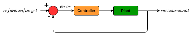
Proportional-Integral-Derivative (PID) controller is an example of a feedback controller. A feedback controller is a type of controller that uses the output of some system to measure error signals or deviations from some target or reference point, and uses these error signals to alter the control signals so that the errors are minimized. Intuitively, if we know how much we deviate from our target, we should take an action that will reduce the error. The figure below is the commonly used diagram to illustrate a feedback controller.
For example, say we have a mobile robot driving on a road, which we can control by changing its linear velocity and angular velocity, and has a sensor that can measure how far the robot is from the center of the lane. The goal is to make sure the robot stays in the middle of the lane. As a controller designer, whenever the robot deviates from the middle of the lane, we may want to adjust the angular velocity such that the robot turns toward the middle of the lane. The question is: by how much?
The name proportional-integral-derivative comes from the fact that the controller adjusts the control signals proportionally to the error at a particular time step \(e(t)\). In addition, the controller also considers the integral of the error over time, and the derivative of the error at each time step (i.e., how the error changes over time). Concretely, the control command \(u(t)\) is calculated by considering the combination of these three components:
\[u(t) = K_p \cdot e(t) + K_i \cdot \int_0^t e(t) dt + K_d \cdot \frac{de(t)}{dt}\]where \(K_p\), \(K_i\), and \(K_d\) denote the proportional, integral, and derivative parameters, respectively. Increasing the proportional term will decrease the rise time (i.e., the time it takes for the system to approach the reference point), but at the risk of overshooting. Increasing the derivative term will help to decrease this overshooting by resisting the robot from moving too quickly to reduce the error. Finally, increasing the integral term will help us to eliminate the steady-state error (i.e., the remaining error that we have when the system has converged).
We can adjust the values for \(K_p\), \(K_i\), and \(K_d\) via trial and error. Usually, we can start by only adjusting \(K_p\) while keeping \(K_i = 0\) and \(K_d = 0\) until the controller is able to almost perfectly reach the reference point (i.e., either little bit of overshooting or undershooting). We can then fix the \(K_p\) at this value, and adjust \(K_d\). Once we found the best \(K_d\), we then proceed to adjust \(K_i\), if still needed.
To reinforce our understanding on this topic, I highly recommend watching the video below. Although the video presents the controller in the context of autonomous driving, I find the video explains PID controller in a really intuitive way, and it is also applicable to other applications.
While implementing PID controller may seem simple, there are actually many studies have been conducted on analysing and designing the PID controller. If we just choose the parameters \(K_p\), \(K_i\), and \(K_d\) through trial and error, there is no guarantee that our controller will be stable (e.g., our robot may oscillate or even completely diverge from the reference point). If you take a control theory course, there is a high chance that you will study PID controller in the Laplace form, which allows us to analyse the stability of the controller. There are also techniques like the pole placement and Ziegler-Nichols that can help us to tune our PID controller. We are not going to cover them in this article, but it is always good to be aware and appreciate these works. If you are into control theory, I definitely encourage you to look up these concepts.
Example
Suppose we have \(dt = 0.1\), \(K_p = 10\), \(K_i = 2\), \(K_d = 0.01\). Say we are at \(t = 4\), and
\[e(0) = 3\] \[e(1) = 2\] \[e(2) = 3\] \[e(3) = 5\] \[e(4) = 1\]We can then compute
\[u(4) = (10)(1) + (2)(3 + 2 + 3 + 5 + 1)(0.1) + (0.01)(\frac{1-5}{0.1}) = 12.4\]Follow-Me-Drone with PID Controller
Here is another possible application of PID controller that I worked on a while ago. Combined with a vision-based tracking system that approximates the position of the person in an image with a bounding box at every time step, we can program a drone to follow the tracked person using PID controller! To do this, we first need to define the target or reference point so that we can compute the error signals that will be used by the controller.
First, we can set the center coordinate of the image as the reference point for the center of the bounding box. That is, we want to control the robot such that the bounding box center is located at the center of the image. These error signals allow us to adjust the yaw (i.e., left/right rotation) and elevation (i.e., up/down movement) rate of the drone to maintain the bounding box location. In addition to this, assuming the size of the bounding box correlates well with how far the drone is from the target, we can also set a reference size for the bounding box as a target. This error signal allows us to adjust the pitch (i.e., forward/backward motion) rate of the drone to maintain the distance between the drone and the tracked object. If we assume these three error signals to be independent from each other, we can use three independent controllers for controlling the yaw, elevation, and pitch. This means, we have in total nine different parameters to be tuned: \(K_p^{yaw}\), \(K_i^{yaw}\), \(K_d^{yaw}\), \(K_p^{elevation}\), \(K_i^{elevation}\), \(K_d^{elevation}\), \(K_p^{pitch}\), \(K_i^{pitch}\), and \(K_d^{pitch}\).
The results can be seen in the video below. In this project, we used the GOTURN (Held et al., 2016) as the object tracker. Nevertheless, other types of trackers can also be used.
Summary
That is all for PID controller. Though it may seem simple, PID controller is powerful and definitely one of the most commonly used controller today. Next time, we will discuss a more advanced controller like the Linear Quadratic Regulator (LQR). Please feel free to send me an email if you have questions, suggestions, or if you found some mistakes in this article. Until next time!
References
Aerospace Controls Laboratory @MIT. Controlling Self Driving Cars. YouTube, 2015. URL.
David Held, Sebastian Thrun, and Silvio Savarese. Learning to Track at 100 FPS with Deep Regression Networks. European Conference on Computer Vision (ECCV), 2016.
Next: Feedback Control with Linear Quadratic Regulator (LQR)