Robotik - Ep.5: Feedback Control with Linear Quadratic Regulator (LQR)
Previous: Intro to Control and Proportional-Integral-Derivative (PID) Controller
We covered the Proportional-Integral-Derivative (PID) controller in the previous post. In this post we will discuss about another controller called the Linear Quadratic Regulator (LQR).
Linear Quadratic Regulator (LQR)
Just like PID, the Linear Quadratic Regulator (LQR) is also considered as a feedback controller. Nevertheless, LQR computes the control signals by modelling it as an optimization problem. That is, it tries to compute control signals that minimizes some cost function.
Consider a linear system:
\[\dot{s} = As + Bu\]where \(s\) is an \(n\)-dimensional vector that represents the state of the system, and \(u\) is an \(m\)-dimensional vector that represents the control signal. Here, \(A\) and \(B\) are \(n\)-by-\(n\) and \(m\)-by-\(m\) matrices, respectively, that describes the dynamics of the system. Say we also have a goal state \(s_g\) that we want to reach. Our job is to find a sequence of control signals \(u\) that will take us to this goal state.
The assumption we make in LQR is that the controller is a linear controller. In turns out that in most cases, a simple linear controller in the form of \(u = -ks\) works well to solve this problem. The question now is: what is \(k\) and how do we find \(k\) that can achieve our goal?
First, we need to define a cost function that quantify the performance of the controller. In LQR we define the cost function as a quadratic cost function:
\[C = \int_{t = 0}^{t = H} ((s_t - s_g)^T Q (s_t - s_g) + u_t^T R u_t) dt\]where \(t\) denotes the time, while \(Q\) and \(R\) are positive definite matrices where off-diagonal elements in the matrix are all 0. Intuitively, each of the diagonal elements in \(Q\) reflect how much we care about a particular error signal. On the other hand, each element in \(R\) reflect how much we care about performing a particular action. In practice, \(Q\) and \(R\) are something that we as the controller designer manually choose depending on how we want the systems to perform (this will become clearer in the example section below). At this point the name ‘‘LQR’’ actually starts to make sense. It comes from the fact that: (1) we assume a linear controller, we use a quadratic cost function, and (3) we aim to regulate the system.
We can also write the cost function in a non-matrix form, which may look more clear for some people. For a system with \(n\)-dimensional states and \(m\)-dimensional control signal where:
\[\small s_t = \begin{bmatrix} s_t^1 \\ s_t^2 \\ \vdots \\ s_t^n \end{bmatrix} \ \ \ \ s_g = \begin{bmatrix} s_g^1 \\ s_g^2 \\ \vdots \\ s_g^n \end{bmatrix} \ \ \ \ u_t = \begin{bmatrix} u_t^1 \\ u_t^2 \\ \vdots \\ u_t^m \end{bmatrix}\] \[\small Q = \begin{bmatrix} Q_{11} & \cdots & Q_{1n} \\ \vdots & \ddots & \vdots \\ Q_{n1} & \cdots & Q_{nn} \\ \end{bmatrix} \ \ \ \ R = \begin{bmatrix} R_{11} & \cdots & R_{1m} \\ \vdots & \ddots & \vdots \\ R_{m1} & \cdots & R_{mm} \\ \end{bmatrix}\]the cost written in a non-matrix form is essentially:
\[C = \int_{t = 0}^{t = H} (s_t^1 - s_g^1)^2 Q_{11} + \cdots + (s_t^n - s_g^n)^2 Q_{nn} + (u_t^1)^2 R_{11} + (u_t^2)^2 R_{22} + \cdots + (u_t^m)^2 R_{mm}\]Note: \(s_t^i\) denotes the \(i\)-th element of the state \(s_t\) at time \(t\).
Now that we have defined the cost function, our job is to find the best sequence of \(u\) that minimizes this cost. Since we assume linear controller in the form of \(u = -ks\), this is the same as finding the best \(k\). There are multiple ways to solve for \(k\). One of the common methods to solve for \(k\) that we learn when talking about LQR is by first solving what is known as the Riccati equation. Practically speaking, there are libraries such as scipy or MATLAB that can help us to solve for the Riccati equation and \(k\). I am not going to go through the derivation here, but we can get a closed-form solution that looks something like:
\[k_h = -(R + B^T P_{h+1} B)^{-1}B^T P_{h+1} A, \ \textrm{for h = H,...,0}\] \[P_{h} = Q + k_h^T R K_h + (A + B K_h)^T P_{h+1}(A + B K_h)\] \[P_{H} = Q\]For now, let’s assume we can get \(k\) using existing libraries given \(A\), \(B\), \(Q\), and \(R\) matrices. For those who are interested to know more about it, I encourage you to look it up. I also highly recommend watching the video below from to have a better intuition of how LQR works.
Notice that so far, we have been assuming that our system is linear and can be easily written in the form of \(\dot{s} = As + Bu\). In the case where we have a non-linear system, we need to first linearize it around a fixed point, and then compute for \(A\) and \(B\). We will encounter this in the example below. Let’s take a look at the example.
Example
One of the most common examples to learn LQR is the problem of controlling an inverted pendulum. The figure below illustrates the system.
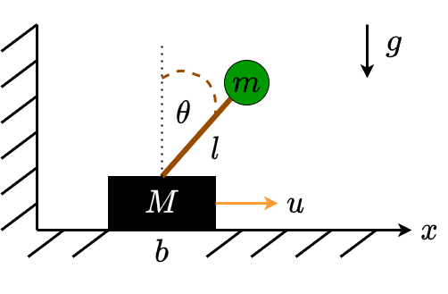
The state of the system is defined by the cartpole’s horizontal position \(x\), cartpole velocity \(\dot{x}\), pendulum angle \(\theta\), the rate of change of pendulum angle (i.e., angular velocity) \(\dot{\theta}\). Our main goal is to apply force \(u\) on the cart that will move it in left or right direction, such that the pendulum is in upright position (i.e., \(\theta = 0\)). Here, \(b\) and \(g\) denotes the friction coefficient and gravitational force, respectively.
\[\small s_t = \begin{bmatrix} x \\ \dot{x} \\ \dot{\theta} \\ \theta \end{bmatrix} \ \ \ \ u_t = \begin{bmatrix} u \\ \end{bmatrix}\]The dynamics of the system is given as:
\[\ddot{x} = \frac{2m\mathcal{l}\dot{\theta}^2 \sin \theta + 3 m g \sin \theta \cos \theta + 4u - 4b\dot{x} } {4M + 4m - 3m \cos^2 \theta}\] \[\ddot{\theta} = \frac{-3ml\dot{\theta}^2 \sin \theta \cos \theta - 6Mg \sin \theta - 6mg \sin \theta - 6u \cos \theta + 6b \dot{x} \cos \theta}{ 4\mathcal{l}M + 4\mathcal{l}m - 3\mathcal{l}m \cos^2 \theta }\]Assuming \(u = - ks\), we want to calculate the control policy \(k\) that minimizes the cost function:
\[C = \int_{t = 0}^{t = H} ((s_t - s_g)^T Q (s_t - s_g) + u_t^T R u_t) dt\]In this example, we have four types of error signals: (1) error in horizontal position, (2) error in horizontal velocity, (3) error in pendulum angle, and (4) error in angular velocity of the pendulum. In addition to this, the cost is also a function of the action \(u\). How do we determine \(Q\) and \(R\)? Well, this depends on how we want the system to behave. In this example, we may want to prioritize the error in pendulum angle, thus we can put a larger weight on this error signal. If we do not care about the position of the cartpole, we can set the weight in \(Q\) that corresponds to this error signal to be \(0\). With the same logic, we can also determine the weights for both the errors in \(\dot{x}\) and \(\dot{\theta}\). As for \(R\), we can think of it as how much energy or force we are willing to spend to reach the target. Larger weights in \(R\) means that we are not willing to spend too much energy.
Since the system is a non-linear one, we first need to linearize the system around a fixed point (e.g., when \(\theta = 0, \dot{\theta} = 0, \dot{x} = 0, x = 0, u = 0\)) to get both the \(A\) and \(B\) matrices. Recall that:
\[\dot{s} = As + Bu\]where
\[\small s = \begin{bmatrix} x \\ \dot{x} \\ \dot{\theta} \\ \theta \end{bmatrix}\]thus
\[\small \dot{s} = \begin{bmatrix} \dot{x} \\ \ddot{x} \\ \ddot{\theta} \\ \dot{\theta} \end{bmatrix}\]Now, let’s denote
\[\dot{x} = f_1(s,u)\] \[\ddot{x} = f_2(s,u)\] \[\ddot{\theta} = f_3(s,u)\] \[\dot{\theta} = f_4(s,u)\]our \(A\) and \(B\) matrix will be
\[\small A = \begin{bmatrix} \frac{\partial f_1}{\partial x} & \frac{\partial f_1}{\partial \dot{x}} & \frac{\partial f_1}{\partial \dot{\theta}} & \frac{\partial f_1}{\partial \theta} \\ \frac{\partial f_2}{\partial x} & \frac{\partial f_2}{\partial \dot{x}} & \frac{\partial f_2}{\partial \dot{\theta}} & \frac{\partial f_2}{\partial \theta} \\ \frac{\partial f_3}{\partial x} & \frac{\partial f_3}{\partial \dot{x}} & \frac{\partial f_3}{\partial \dot{\theta}} & \frac{\partial f_3}{\partial \theta} \\ \frac{\partial f_4}{\partial x} & \frac{\partial f_4}{\partial \dot{x}} & \frac{\partial f_4}{\partial \dot{\theta}} & \frac{\partial f_4}{\partial \theta} \\ \end{bmatrix} \ \ \ \ B = \begin{bmatrix} \frac{\partial f_1}{\partial u} \\ \frac{\partial f_2}{\partial u} \\ \frac{\partial f_3}{\partial u} \\ \frac{\partial f_4}{\partial u} \\ \end{bmatrix}\]where each of the partial derivatives is evaluated at the fixed point. So, for example, since
\[f_2 = \ddot{x} = \frac{2m\mathcal{l}\dot{\theta}^2 \sin \theta + 3 m g \sin \theta \cos \theta + 4u - 4b\dot{x} } {4M + 4m - 3m \cos^2 \theta}\]we get
\[\frac{\partial f_2}{\partial x} = 0\] \[\frac{\partial f_2}{\partial \dot{x}} = \frac{-4b}{4M + 4m - 3m\cos^2\theta} \biggr\rvert_{\theta = 0, \dot{\theta} = 0, \dot{x} = 0, x = 0, u = 0} = \frac{-4b}{4M + m}\] \[\frac{\partial f_2}{\partial \dot{\theta}} = \frac{2(2ml\dot{\theta} \sin \theta)}{4M + 4m - 3m\cos^2\theta} \biggr\rvert_{\theta = 0, \dot{\theta} = 0, \dot{x} = 0, x = 0, u = 0} = 0\] \[\frac{\partial f_2}{\partial \theta} = \frac{3mg}{4M + m}\]To keep this article short, we will skip the calculation for the rest of the partial derivatives. It is also a good exercise for you to try on your own :). If you do it correctly, you will get
\[\small A = \begin{bmatrix} 0 & 1 & 0 & 0 \\ 0 & \frac{-4b}{4M + m} & 0 & \frac{3mg}{4M + m} \\ 0 & \frac{6b}{4M\mathcal{l} + m\mathcal{l}} & 0 & \frac{-6Mg - 6mg}{4M\mathcal{l} + m\mathcal{l}} \\ 0 & 0 & 1 & 0 \\ \end{bmatrix} \ \ \ \ B = \begin{bmatrix} 0 \\ \frac{4}{4M + m} \\ \frac{-6}{4M\mathcal{l} + m\mathcal{l}} \\ 0 \\ \end{bmatrix}\]Once we have \(A\) and \(B\) we can then solve for \(k\) that minimizes the cost function. As long as the error is not too large, the controller should be able to balance the pendulum!
Summary
To summarize, given a linear or non-linear system, LQR works as following:
-
Get \(A\) and \(B\) matrices. If the system is linear, we write the system in the form of \(\dot{s} = As + Bu\). Else if the system is non-linear, we first linearize the system around a fixed point, and then calculate the Jacobian to get \(A\) and \(B\).
-
Once we have \(A\) and \(B\), we can sometimes determine if the system is controllable or not by just looking at them. In other cases, a more appropriate techniques to determine controllability may be needed.
-
We define a quadratic cost function \(C = \int_{t = 0}^{t = H} ((s_t - s_g)^T Q (s_t - s_g) + u_t^T R u_t) dt\), and manually define \(Q\) and \(R\) matrices.
-
We then assume a linear controller \(u = - ks\), and solve for the best \(k\) that minimizes the cost function.
That is all for LQR! Please feel free to send me an email if you have questions, suggestions, or if you found some mistakes in this article. Until next time!
References
Steve Brunton. Linear Quadratic Regulator (LQR) Control for the Inverted Pendulum on a Cart [Control Bootcamp]. YouTube, 2017. URL.