Robotik - Ep.3: Multi-query Motion Planning with Probabilistic RoadMaps (PRM)
Previous: Intro to Motion Planning and Rapidly-exploring Random Tree (RRT)
In the previous post, we discussed about motion planning and the Rapidly-exploring Random Tree (RRT) algorithm. RRT is an algorithm that only applies in single-query applications. This means that we need to run RRT from scratch everytime we want to solve a motion planning problem. In other words, any plans generated by RRT are not reusable in the future. In multi-query applications, we only build the graph once, and use the same graph multiple times to solve different motion planning queries. Probabilistic RoadMaps (PRM) is an algorithm that we can use for multi-query applications.
Probabilistic RoadMaps (PRM)
Similar to Rapidly-exploring Random Tree (RRT), Probabilistic RoadMaps (PRM) is an algorithm that builds a graph to perform motion planning. PRM also makes similar assumptions as in RRT: we know the map of the environment, we are able to check the distance between two states, and we can check if obstacles exist in between two nodes. We will mostly talk about the simplified version of PRM called the sPRM, following Karaman & Frazzoli (2011).
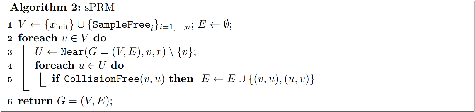
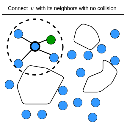
The sPRM algorithm works as the following. Given an initial state \(x_{init}\), we first define a set of vertices \(V\) and put \(x_{init}\) in it. We then samples \(n\) random states and put them all in \(V\), and start with an empty set of edges \(E\). For every vertice \(v \in V\), we find a set of vertices (denoted as \(U\)) whose distance is less than some radius \(r\) from \(v\). Then for every vertice \(u \in U\), we check if there are obstacles between \(u\) and \(v\). If there are no obstacles, we create edges from \(u\) to \(v\), and vice-versa. PRM returns the graph that contains the initial state \(x_{init}\) and random states that we sample from the environment. If we know where we are in the graph (i.e., we know the state of our robot), then we can find the path from where the robot is, to any of the nodes in the graph, as long as the path exists. The PRM algorithm is shown below (Karaman & Frazzoli, 2011) (Note: for those who are not familiar with the notation, \(\setminus \{v\}\) means to not include the node \(v\) into \(U\)).
There are other PRM variants like PRM*, but let’s leave it for future posts. For now, let’s take a look at an example of how PRM works.
Example
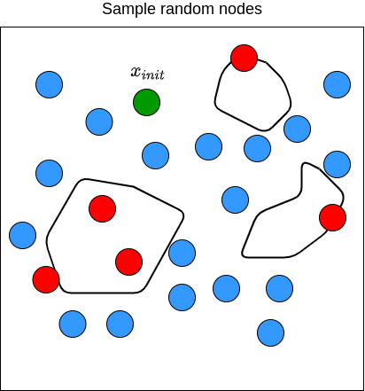
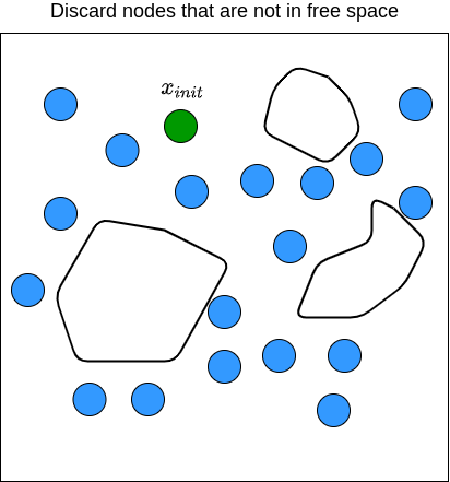
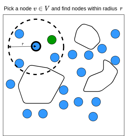
Here is the step-by-step visualization of how PRM works in 2D space where the state is defined by \((x,y)\) coordinates:
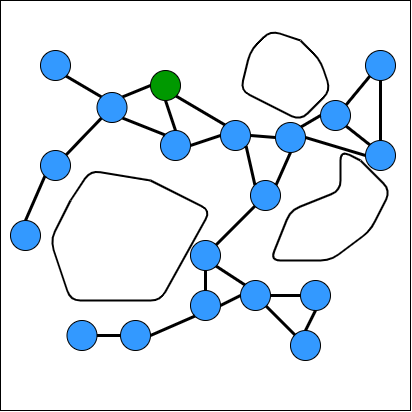
We then repeat these processes until we have gone through all the samples \(v \in V\). The figure below illustrates what the end results of PRM may look like.
Summary
That is it! Now we have seen algorithm to solve multi-query motion planning. Later on, we will discuss about more optimal variants of both RRT and PRM. Please feel free to send me an email if you have questions, suggestions, or if you found some mistakes in this article. Until next time!
References
Sertac Karaman and Emilio Frazzoli. Sampling-based Algorithms for Optimal Motion Planning. The International Journal of Robotics Research, 2011.
Next: Intro to Control and Proportional-Integral-Derivative (PID) Controller