Robotik - Ep.1: Intro to State Estimation and Bayes Filter
In this post, we will learn about state estimation problem, and a method to solve it called Bayes filter. A state describes the condition of our robot at a specific time. For example, a location of a robot on a 2D plane can be considered as a state. If we are interested in where the robot is facing, we can also define the state to contain both the position and the orientation of the robot. In real world, we usually do not know the exact state of the robot. Instead, we need to infer the state of the robot from its noisy sensors. State estimation is thus the problem of estimating the state of our robot from noisy sensors data.
In addition, we can also incorporate the knowledge that we have about the motion of the robot. The intuition is that, if we know where the robot currently is, knowing the action that the robot took and how the state of the robot should change due to that action (we call this a motion model) should give us information about the state of the robot in the next time step. Before we jump in to the main course, let’s start by reviewing basics of probability and Bayes rule. Feel free to skip it if you feel comfortable with these concepts already.
Probability and Bayes Rule
Probability is a measure of how likely an event to occur. For example, if we flip a fair coin, the probability of getting a “head” is equal to the probability of getting a “tail”. To denote this mathematically, we say \(p(X = head) = p(X = tail) = 0.5\), where \(X\) is a random variable (i.e., a variable whose value is random). Let’s also denote the set of possible events as \(\Omega\) (e.g., in the coin flip example, the random variable can be either “head” or “tail”, thus \(\Omega = \{head, tail\}\)) and the event as \(x\), where \(x \in \Omega\). To simplify notation, we sometimes will write \(p(X = x)\) as \(p(x)\).
There are two types of random variables. The first is discrete random variable, where the possible values for the random variable is countable, just like the coin flip example. The second type is continuous random variable, where the possible values is non-countable. The sum of probability of all of the possible events for discrete random variables must equal to 1. In other words, \(\sum_{x \in \Omega} p(x) = 1\). Whereas with continuous random variables, the integration of all possible events must equal to 1. In other words, \(\int p(x) dx = 1\). While it makes sense for us to query \(p(X = x)\) when \(X\) is a discrete random variable, querying for \(p(X = x)\) is not valid when \(X\) is a continuous random variable since there are infinite number of possible states. Instead, the valid question to ask is the probability of \(X\) to fall between two values \(p(a < x < b)\).
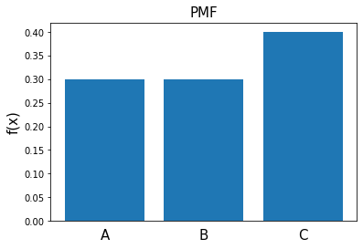
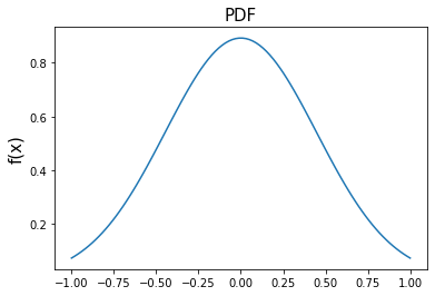
Continuous random variables are characterized by probability density function (PDF), while discrete random variables are characterized by probability mass function (PMF). We often refer to these as the probability distribution, since they both tell us how the probability of all possible events are distributed. The figure below illustrates the difference. Note that \(f(x)\) directly translates to \(p(X = x)\) in PMF, while it is not the case in PDF. Remember, with continuous random variables, we want \(\int_a^b p(x) dx = 1\), and sum behaves differently than integration.
Joint probability is the probability of multiple events occuring together. For example, if we consider two coin flips, we may want to know what the probability is for both coins to be “head”. We denote this as \(p(X = x, Y = y)\) or simply \(p(x, y)\). If the outcome of \(X\) does not affect the outcome of \(Y\) and vice-versa, we call \(X\) and \(Y\) to be independent. If \(X\) and \(Y\) are independent, then \(p(x, y) = p(x) p(y)\). In our coin flip example, the random variables are independent since the outcome of the first coin clip does not affect the second coin flip.
The conditional distribution \(p(x \vert y)\) (assuming two random variables) is the probability of event \(x\) to happen, given the fact that event \(y\) is occuring. The conditional distribution is also defined as \(p(x \vert y) = \frac{p(x,y)}{p(y)}\).
Finally, Bayes rule enables us to relate \(p(x \vert y)\) with \(p(y \vert x)\). It states that \(p(y \vert x) = \frac{p(x \vert y) p(y)}{p(x)}\). We can also write the Bayes rule as \(p(y \vert x) = \eta p(x \vert y)p(y)\), where \(\eta\) is a normalization term.
Measurement and Motion Models
As previously mentioned, we have to be able to deal with data from noisy sensors. Measurement model or a sensor model represents the probability of a measurement given a particular state. For example, if we have a light sensor that detects whether a light is “on” or “off”, we may have a sensor model that looks like the following:
\[\small p(measurement \vert light) = \begin{bmatrix} p(measurement = on \vert light = on) & p(measurement = on \vert light = off) \\ p(measurement = off \vert light = on) & p(measurement = off \vert light = off) \end{bmatrix}\]From now on, we will denote state and measurement at time \(t\) as \(x_t\) and \(z_t\), respectively.
Motion model is a model that describes how a state transitions to another after an action is taken. For example, consider a robot is initially located at \((X = x, Y = y)\), where \(+x\) and \(+y\) point to east and north, respectively. Also assume that we have the ability to control the robot by commanding it to move east/west/north/south by one unit. If we command the robot to move east, then we expect the robot to arrive at \((X = x + 1, Y = y)\). However, since robot motion is also not perfect in the real world, the robot may end up in a slightly different location. Perhaps at \((X = x + 0.8, Y = y + 0.01)\) or maybe \((X = x + 1.05, Y = y - 0.01)\). Thus, we should also define the motion of the robot as a probabilistic model. That is, instead of saying the probability of the robot being at \((X = x + 1, Y = y)\) given that the robot started at \((X = x, Y = x)\) and moved east is equal to 1, we should model the transition by considering the distribution of all possible states that the robot may end up at (i.e., \(p(x_{t} \vert x_{t-1}, u_{t-1})\), where \(u_{t-1}\) denotes the action the robot took at time \(t-1\)).
Now that we have the tools, we can move on and look into how to perform state estimation with something called Bayes filter.
State Estimation with Bayes Filter
There are two types of estimation problems that we can consider: smoothing and filtering. Smoothing is a problem where we are interested to compute the sequence of estimated states after we collect a sequence of sensor measurements and actions. In other words, we would like to know:
\[p(x_{0:T} \vert z_{0:T},u_{0:T-1})\]where \(T\) denotes the time where the sequence ended.
Filtering deals with state estimation online as we execute an action and take a measurement. That is, we would like to know the probability of being in a particular state at current time step \(t\) given past actions and measurements (we also call this as the belief):
\[p(x_{t} \vert z_{0:t},u_{0:t-1})\]Bayes filter is a method of filtering. To work with Bayes filter, we first need to make two assumptions. The first is to assume that the current state is conditonally independent of previous sequence of states and controls given previous state. That is, \(p(x_{t} \vert x_{o:t-1}, u_{0:t-1}) = p(x_t \vert x_{t-1}, u_{t-1})\). This assumption is known widely as the Markov assumption. The second assumption is that the world is static, or given the current state, the sensor measurement is conditonally independent of past measurements and actions. In other words, \(p(z_t \vert x_t, u_{0:t-1}, z_{0:t-1}) = p(z_t \vert x_t)\).
To have a better understanding of Bayes filter, let’s take a look at how it was derived. That being said, feel free to skip it and only look at the final results if you do not find it interesting. The derivation of Bayes filter goes as following (adapted from slides made by David Meger for his Intelligent Robotics class at McGill):
\[\begin{eqnarray} bel(x_t) &=& p(x_t \vert u_{0:t-1},z_{0:t}) \\ &=& \eta p(z_t \vert x_t,u_{0:t-1},z_{0:t-1}) p(x_t \vert u_{0:t-1},z_{0:t-1}) \quad \quad \quad \quad \quad \quad \quad \quad \quad \quad \quad \ \ \ \textrm{conditional Bayes rule} \\ &=& \eta p(z_t \vert x_t) p(x_t \vert u_{0:t-1}, z_{0:t-1}) \quad \quad \quad \quad \quad \quad \quad \quad \quad \quad \quad \quad \quad \quad \quad \quad \quad \ \textrm{static world assumption} \\ &=& \eta p(z_t \vert x_t) \int p(x_t, x_{t-1} \vert u_{0:t-1}, z_{0:t-1}) dx_{t-1} \quad \quad \quad \quad \quad \quad \quad \quad \quad \quad \quad \ \ \textrm{law of total probability} \\ &=& \eta p(z_t \vert x_t) \int p(x_t \vert x_{t-1}, u_{0:t-1}, z_{0:t-1}) p(x_{t-1} \vert u_{0:t-1}, z_{0:t-1}) dx_{t-1} \quad \quad \quad \textrm{conditional distribution} \\ &=& \eta p(z_t \vert x_t) \int p(x_t \vert u_{t-1}, x_{t-1}) p(x_{t-1} \vert u_{0:t-1},z_{0:t-1}) dx_{t-1} \quad \quad \quad \quad \quad \quad \ \textrm{Markov assumption} \\ &=& \eta p(z_t \vert x_t) \int p(x_t \vert u_{t-1}, x_{t-1}) p(x_{t-1} \vert u_{0:t-2},z_{0:t-1}) dx_{t-1} \quad \quad \quad \quad \quad \quad \ u_{t-1} \ \textrm{only affects} \ x_t \\ &=& \eta p(z_t \vert x_t) \int p(x_t \vert u_{t-1}, x_{t-1}) bel(x_{t-1}) dx_{t-1} \quad \quad \quad \quad \quad \quad \quad \quad \quad \quad \quad \textrm{definition of belief} \\ \end{eqnarray}\]We have now derived the Bayes filter. We see that the belief at current time step \(bel(x_t)\) is a function of the belief at the previous time step \(bel(x_{t-1})\). This is useful because we usually know the belief at \(t = 0\), which we call prior belief. To concretize, let’t take a look at an example of how to use it.
Example
Consider a simple robot equipped with a light sensor whose task is to predict whether the light is on or off. In this case, the states are whether the light is “on” or “off”. The light sensor can measure if the robot is in one of these two states. However, the sensor is noisy, and thus cannot be fully trusted. Furthermore, the robot may take the action to turn the light switch.
Given that the measurement model is:
\[\begin{eqnarray} p(z_t \vert x_t) &=& \begin{bmatrix} p(z_t = on \vert x_t = on) & p(z_t = on \vert x_t = off) \\ p(z_t = off \vert x_t = on) & p(z_t = off \vert x_t = off) \end{bmatrix} \\ &=& \begin{bmatrix} 0.9 & 0.4 \\ 0.1 & 0.6 \end{bmatrix} \end{eqnarray}\]and the motion model is:
\[\small \begin{eqnarray} p(x_{t} \vert x_{t-1}, u_{t-1} = turn \ on) &=& \begin{bmatrix} p(x_{t} = on \vert x_{t-1} = on, u_{t-1} = turn \ on) & p(x_{t} = on \vert x_{t-1} = off, u_{t-1} = turn \ on) \\ p(x_{t} = off \vert x_{t-1} = on, u_{t-1} = turn \ on) & p(x_{t} = off \vert x_{t-1} = off, u_{t-1} = turn \ on) \end{bmatrix} \\ &=& \begin{bmatrix} 0.9 & 0.8 \\ 0.1 & 0.2 \end{bmatrix} \end{eqnarray}\] \[\small \begin{eqnarray} p(x_{t} \vert x_{t-1}, u_{t-1} = turn \ off) &=& \begin{bmatrix} p(x_{t} = on \vert x_{t-1} = on, u_{t-1} = turn \ off) & p(x_{t} = on \vert x_{t-1} = off, u_{t-1} = turn \ off) \\ p(x_{t} = off \vert x_{t-1} = on, u_{t-1} = turn \ off) & p(x_{t} = off \vert x_{t-1} = off, u_{t-1} = turn \ off) \end{bmatrix} \\ &=& \begin{bmatrix} 0.3 & 0.2 \\ 0.7 & 0.8 \end{bmatrix} \end{eqnarray}\]and the prior:
\[bel(x_0) = \begin{bmatrix} bel(x_0 = on) \\ bel(x_0 = off) \end{bmatrix} = \begin{bmatrix} 0.5 \\ 0.5 \end{bmatrix}\]what is the belief after 1 time step (i.e., \(bel(x_1)\)) where \(u_0 = turn \ on\) and \(z_1 = on\)?
We can compute this by first predicting what the next state will be without considering the measurement. We refer this as the state prediction step. This is exactly the integral term in \(bel(x_t) = \eta p(z_t \vert x_t) \int p(x_t \vert u_{t-1}, x_{t-1}) bel(x_{t-1}) dx_{t-1}\). Let’s denote the integral term as
\[\bar{bel}(x_t) = \int p(x_t \vert u_{t-1}, x_{t-1}) bel(x_{t-1}) dx_{t-1}\]Since the example deals with discrete random variables and actions, we instead compute the sum instead of the integral:
\[\bar{bel}(x_t) = \sum p(x_t \vert u_{t-1}, x_{t-1}) bel(x_{t-1})\]Concretely, we want to compute \(\bar{bel}(x_1 = on)\) and \(\bar{bel}(x_1 = off)\):
\[\begin{eqnarray} \bar{bel}(x_1 = on) &=& p(x_1 = on \vert x_{0} = on, u_{0} = turn \ on) bel(x_{0} = on) \\ &\quad& + p(x_1 = on \vert x_{0} = off, u_{0} = turn \ on) bel(x_{0} = off) \\ &=& (0.9)(0.5)+ (0.8)(0.5) \\ &=& 0.85 \end{eqnarray}\] \[\begin{eqnarray} \bar{bel}(x_1 = off) &=& p(x_1 = off \vert x_{0} = on, u_{0} = turn \ on) bel(x_{0} = on) \\ &\quad& + p(x_1 = off \vert x_{0} = off, u_{0} = turn \ on) bel(x_{0} = off) \\ &=& (0.1)(0.5)+ (0.2)(0.5) \\ &=& 0.15 \end{eqnarray}\]We then consider the measurement and use it to update the state prediction. This is called the measurement update step. Recall that
\[bel(x_t) = \eta p(z_t \vert x_t) \bar{bel}(x_t)\]thus, knowing that \(z_1 = on\) gives us
\[\begin{eqnarray} bel(x_1 = on) &=& \eta p(z_1 = on \vert x_1 = on) \bar{bel}(x_1 = on) \\ &=& \eta (0.9) (0.85) = \eta 0.765 \end{eqnarray}\] \[\begin{eqnarray} bel(x_1 = off) &=& \eta p(z_1 = on \vert x_1 = off) \bar{bel}(x_1 = off) \\ &=& \eta (0.4) (0.15) = \eta 0.06 \end{eqnarray}\]Then we can compute \(\eta\):
\[\eta = \frac{1}{0.765 + 0.06} = 1.212\]Finally, we have
\[bel(x_1 = on) = (1.212) (0.765) = 0.927\] \[bel(x_1 = off) = (1.212) (0.06) = 0.073\]Summary
Now we know how to use Bayes filter to solve the state estimation problem. We will see later that the understanding of Bayes filter will also be useful in understanding other techniques such as particle filter and Kalman filter. Please feel free to send me an email if you have questions, suggestions, or if you found some mistakes in this article.
References
Sebastian Thrun, Wolfram Burgard, and Dieter Fox. Probabilistic Robotics (Intelligent Robotics and Autonomous Agents). The MIT Press, 2005.
David Meger. Reasoning Under Uncertainty. PowerPoint Presentation, 2020. URL https://www.cim.mcgill.ca/~dmeger/comp765/index2020.html.
Next: Intro to Motion Planning and Rapidly-exploring Random Tree (RRT)