Robotik - Ep.2: Intro to Motion Planning and Rapidly-exploring Random Tree (RRT)
Previous: Intro to State Estimation and Bayes Filter
One of the most common paradigms in robotics is the sense-plan-act paradigm. In this paradigm, a robot senses its surroundings using its sensors, make a plan to achieve its goal based on what it sensed, and then execute its plan by taking actions. A plan is a path (i.e., a sequence of states) that takes a robot from its current state to a goal state. Ideally, a path should also respect the robot’s kinematics and dynamics. For example, a feasible plan for an autonomous vehicle should not include a path that requires the vehicle to move sideways.
There are various types of planners. These include behavior-based planner, graph-based planner, cell decomposition planner, and others. In this post, we will discuss about a particular sampling-based motion planning algorithm called Rapidly-exploring Random Tree (RRT).
Rapidly-exploring Random Tree (RRT)
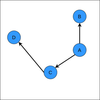
Rapidly-exploring Random Tree (RRT) is a motion planning algorithm that find the feasible path from an initial state to a goal state by building a graph. In this context, a graph is a data structure that represents how states are related to each other. For example, if we are in state \(A\), a graph \(G\) may tell us which other states are reachable from state \(A\). Here, we call the states to be the nodes or vertices of the graph. The relations between states are called the edges of the graph, and usually represented as lines or arrows between nodes. When we see arrows, it usually means that the we have a directed graph. For example, if we see \(A \rightarrow B\), it means that we can reach state \(B\) from \(A\), but not from \(B\) to \(A\). The edges of a graph can mean different things like the probability to reach other states. For now, let’s talk about directed graph where the nodes represent states, and the edges represent what states are reachable from the others. An illustration of a graph is shown below.
First, let’s talk about the assumptions made in RRT. RRT assumes that we know the map of the environment and the dynamics of the robot. It also assumes that we are able to check the distance between two states, and if obstacles exist in between two states. Note that these assumptions are not necessarily realistic. Nevertheless, they give us a good starting point, and if we have a robotics system with known dynamics that can build a map, we can definitely use RRT to solve our motion planning problems.
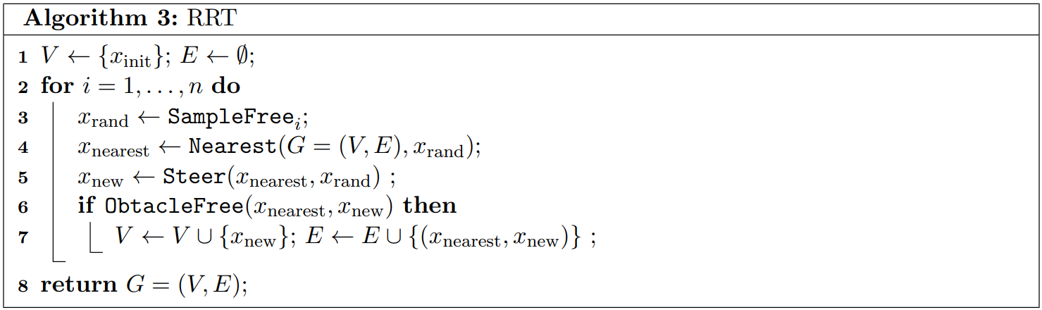
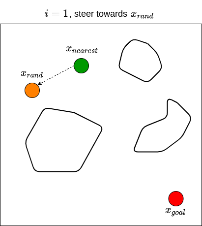
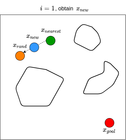
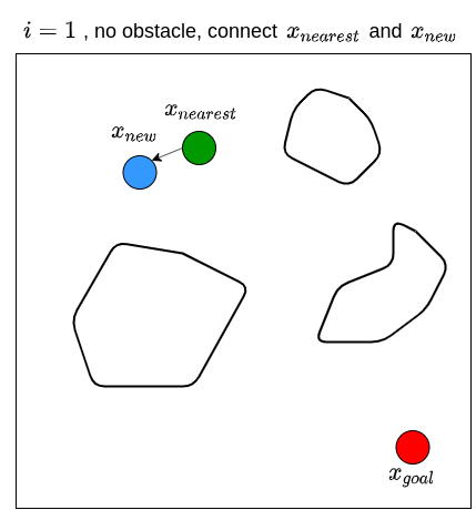
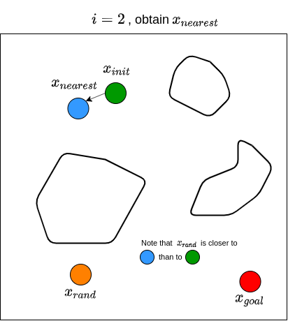
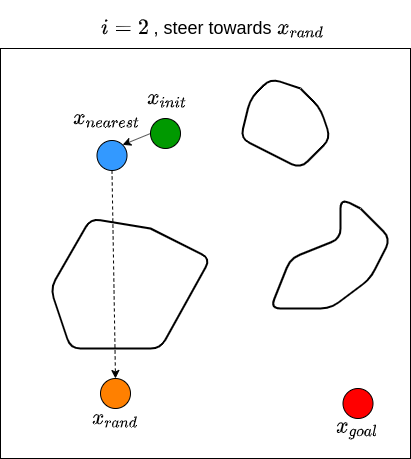
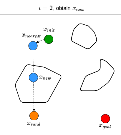
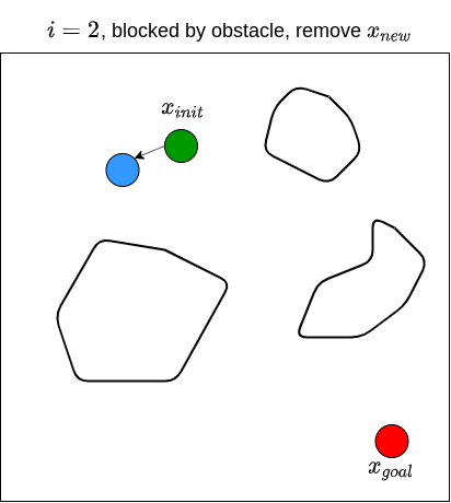
Let’s now see how RRT actually works. Given a goal state \(x_{goal}\) and an initial state \(x_{init}\), we first define a set of vertices \(V\) and put \(x_{init}\) in it. We also start with an empty set of edges \(E\). That is, we start with a graph that contains only one node (i.e., \(x_{init}\)) with no edges. We then sample a random state \(x_{rand}\), and find the state (i.e., node) from the existing graph that is nearest to \(x_{rand}\); we denote this nearest state \(x_{nearest}\). For example, if the state is defined by \((x,y)\) coordinates in 2D space, then the nearness can be measured by the Euclidean distance between two points. We then attempt to steer from \(x_{nearest}\) towards \(x_{rand}\) to get a new point \(x_{new}\) that is between these two states. For example, one may choose \(x_{new}\) to be a point between \(x_{nearest}\) and \(x_{rand}\) that is \(\epsilon\) away from \(x_{nearest}\), or to be a point in the middle of \(x_{nearest}\) and \(x_{rand}\). Note that the steer function must adhere to the dynamics of the robot. We then check if there are obstacles between \(x_{nearest}\) and \(x_{new}\). If there are no obstacles, we proceed to grow the graph by connecting \(x_{nearest}\) and \(x_{new}\). We then repeat this processes for \(n\) steps, or until we find a path from \(x_{init}\) to \(x_{goal}\). Typically, we stop until we find a state that is close enough to the goal state. RRT returns the graph that connects the initial state to the goal state. Once we have this, we obtain the path by going backwards from goal state to the initial state. The RRT algorithm is shown below (Karaman & Frazzoli, 2011).
Note that the path found using RRT is not necessarily optimal. Nevertheless, RRT guarantess that we can find a path from the start to goal node, if there is any. There are other RRT variants like RRT-Connect and RRT*, but we are not going to cover them here. Furthermore, RRT considers only the single-query case. This means that everytime we need our robot to reach a certain goal state, we need to re-run the RRT algorithm to generate a plan. To deal with multi-query case, we can build the graph with another method called the Probabilistic Roadmaps (PRM). Let’s leave this for later as well.
Example
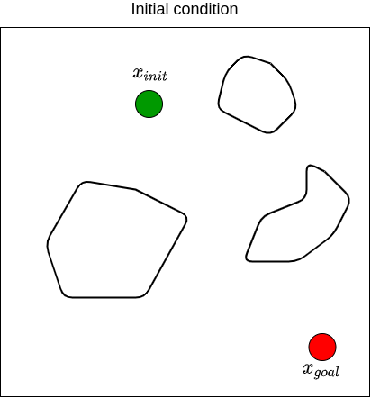
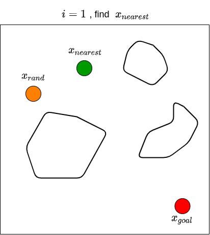
Let’s visualize how RRT works step-by-step in 2D space where the state is defined by \((x,y)\) coordinates:

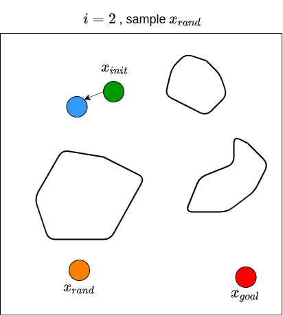
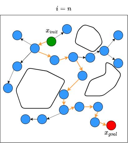
We then repeat these processes for \(n\) steps until we find a state that is close enough to \(x_{goal}\). The figure below illustrates what the end results of RRT may look like, along with the path from \(x_{init}\) to \(x_{goal}\).
Summary
Now we know what motion planning is and how to solve it using RRT. Later, we will discuss other motion planning techniques from different family, as well as more advanced methods like RRT*. Please feel free to send me an email if you have questions, suggestions, or if you found some mistakes in this article. Until next time!
References
Sertac Karaman and Emilio Frazzoli. Sampling-based Algorithms for Optimal Motion Planning. The International Journal of Robotics Research, 2011.
Next: Multi-query Motion Planning with Probabilistic RoadMaps (PRM)