Fundamentals of Large Language Models - Ep.4: Transformer
We have learned now how attention mechanism can significantly improve the performance of a model. Still, there is one major disadvantage left with using RNN-type models: the computation is highly sequential and not parallelizable, so the cost of computation gets worse as the input sequence gets longer. Transformer solves the issues with reccurent models, and has been the backbone of the latest and greatest large language models (LLMs) as of the time of writing this article. Futhermore, transformer has also shown great potential to be used in vision tasks.
Let’s dig in.
Transformer
In terms of architecture, transformer is made up of an encoder and a decoder. The function of the encoder and decoder are pretty much similar with typical RNN-type models such as Seq2Seq. Only now, the computations is no longer highly sequential and unparallelizable. In this article, we will learn new concepts which include positional encoding and multi-head (self) attention. The figure below depicts the transformer architecture.
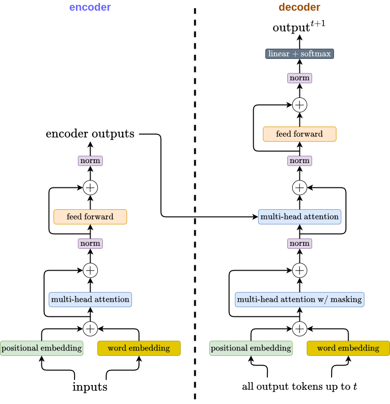
Don’t worry, we’ll take a look at each of the components in detail below.
Positional Encoding
Before going into how the encoder works, first let’s try to understand what positional encoding is. Since transformer does not have any recurrency, there needs to be another mechanism that makes the rest of the model aware of the relative position of the input tokens. To do this, the authors of transformer propose to add positional encoding information into the word embedding. As the name suggests, positional encoding is a way to encode positional information of each input token in the whole input sequence. There are multiple ways to do this, but the authors propose positional encoding based on sine and cosine functions. Let \(D\) be the word embedding dimension, and \(p\) be the token position within the input sequence. The positional encoding is formulated as
\[PE(p,d) = \begin{cases} \sin(p/10,000^{d / D}), & \text{if } d \text{ is even}\\ \cos(p/10,000^{(d-1) / D}), & \text{if } d \text{ is odd}, \end{cases}\]where \(d \in [0, 1, ..., D-1]\). To make it more concrete, here is an example:
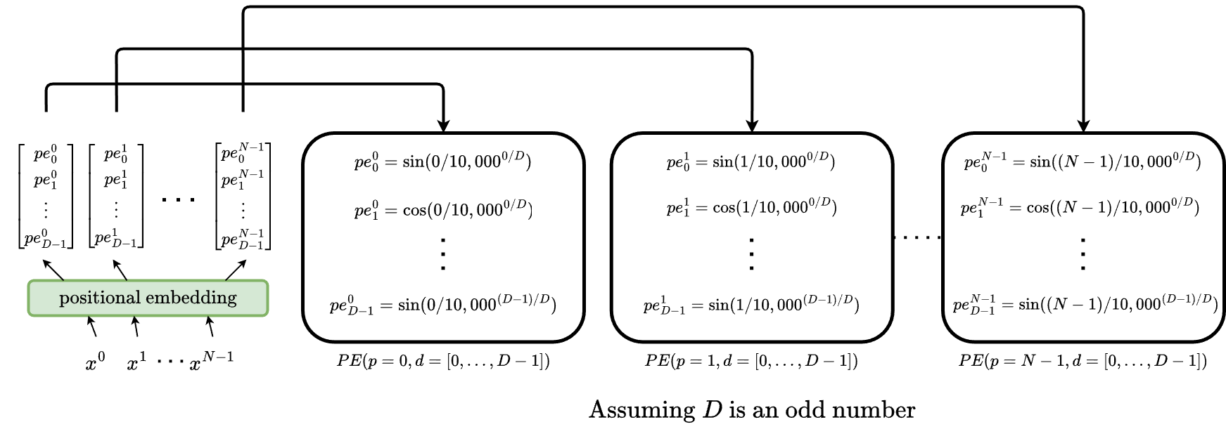
Note that the dimension of each token’s positional embedding is the same as the dimension of the word embedding (i.e., \(D\)), which allows us to sum them up.
Encoder
Let’s now look at how the encoder works starting from the input sequence. The figure below illustrates the encoder.
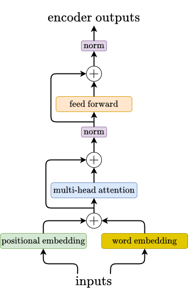
First, given an input sequence containing \(N\) tokens \(x_e = [x_1, x_2, ..., x_N]\), we first embed them individually using typical word embedding layer which produces \(N \times D-\text{dimensional}\) vectors. In parallel, we also generate the positional encoding for each of these \(N\) tokens. We then sum the word embedding together with the positional embedding, which still gives us \(N \times D-\text{dimensional}\) vectors.
Next, we are going to pass these \(N \times D-\text{dimensional}\) vectors into a multi-head attention block. This multi-head attention block is the stage where the model learns how to attend to different parts of the input sequence. First, let’s look more closely at the operations that are happening inside the multi-head attention block below.
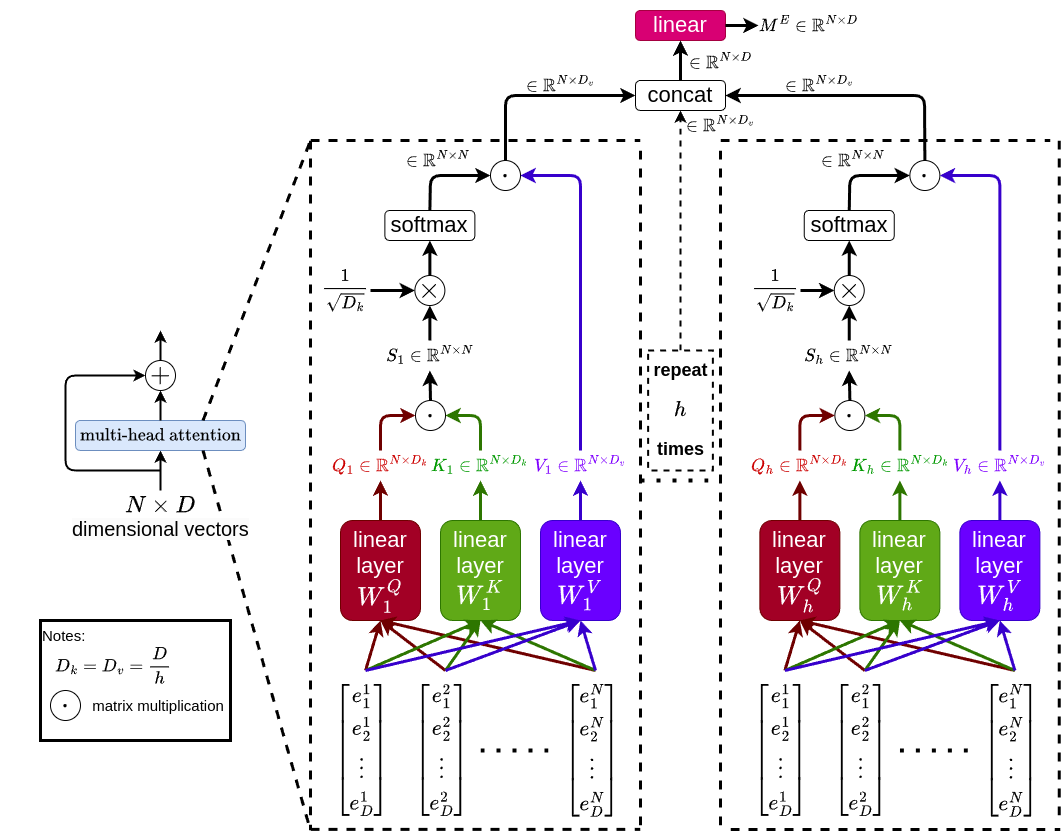
Note that there are \(h\)-layers of multi-head attention. First, for \(i\)-th multi-head attention layer, the input sequence is processed by 3 separate linear layers \(W^Q_i \in \mathbb{R}^{D \times D_k}\), \(W^K_i \in \mathbb{R}^{D \times D_k}\), and \(W^V_i \in \mathbb{R}^{D \times D_v}\), which produces \(Q_i \in \mathbb{R}^{N \times D_k}\), \(K_i \in \mathbb{R}^{N \times D_k}\), and \(V_i \in \mathbb{R}^{N \times D_v}\), respectively. Note that to generate \(Q_i\), \(K_i\), and \(V_i\), we individually multiply each of \(D\)-dimensional input vectors (there are \(N\) of them) with the corresponding weight matrices (i.e., \(W^Q_i\) for \(Q_i\), \(W^K_i\) for \(K_i\), and \(W^V_i\) for \(V_i\)). In other words, \(W^Q_i\), \(W^K_i\), and \(W^V_i\) are “shared” weights. We then multiply \(Q_i\) and \(K_i\) to produce \(S_i \in \mathbb{R}^{N \times N}\), which is the matrix that supposedly capture the relationship between each input tokens. Next, we scale \(S_i\) by multiplying it with \(\frac{1}{\sqrt{D_k}}\), apply softmax to it, and multiply it with \(V_i\). The outputs of each multi-head attention layer are then concatenated, and passed into a final linear layer that produces the multi-head attention output \(M^E \in \mathbb{R}^{N \times D}\).
Finally, we pass \(M^E \in \mathbb{R}^{N \times D}\) to normalization layer, followed by a feedforward layer with a residual connection, and another normalization layer, which gives us the encoder output \(E \in \mathbb{R}^{N \times D}\).
Note that after the initial embedding layers, the encoder essentially maps \(N \times D\) input to \(N \times D\) output. Thus, we can choose to stack the encoder however many times we want if we need to increase the capacity of our transformer.
That wraps up the encoder. Let’s now see how the decoder works!
Decoder
Unlike encoder that can process the whole input sequence in parallel, the decoder is autoregressive in nature: it generates one output token at a time using all the generated tokens from previous time steps.
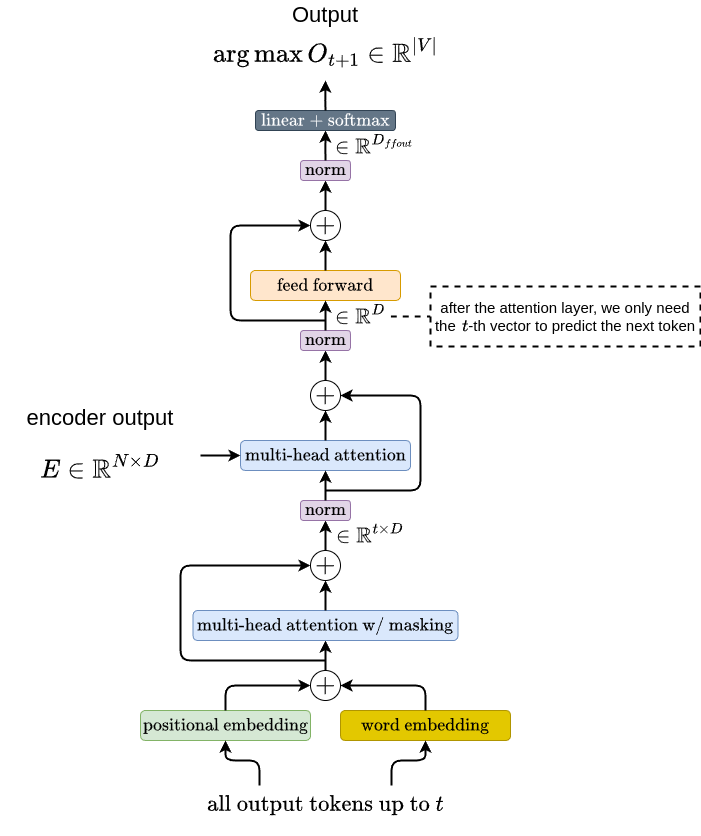
Similar to Seq2Seq, at the very first decoding time step, the input to the decoder \(x_d\) only contains the SOS token. If we assume that \(t\) starts at \(t = 1\), then at each time step, there are \(t\) tokens being passed as the input to the decoder. If we look at the figure above, the way the input is being processed is similar to what we see in the encoder. At each time step, the decoder input \(x_d\) being passed to word embedding and positional embedding layers, and these embeddings are then summed together.
Now the next operation, the multi-head attention with masking, is slightly different than the standard multi-head attention. The difference is that there is an additional masking operation that we need to apply to \(S \in \mathbb{R}^{t \times t}\), where \(S = QK\). The goal of the masking operation is to avoid establishing attention between a token from the past time step to another token in the future time step. The figure below illustrates this operation at \(t = 4\).

Note that we use \(-\infty\) so that those elements will turn into \(0\) after the softmax operation.
After this multi-head attention with masking block, there is another multi-head attention block. Unlike the first one, this one is a standard multi-head attention block like the one we saw in the encoder. But if we look at the decoder illustration above, we saw that we are also passing the output from the encoder to this multi-head attention. What this means is that we will use the output from the first decoder’s multi-head attention with masking block to produce \(Q\), whereas the encoder’s output will be used to produce \(K\) and \(V\).
The rest of the decoder is as straightforward as it looks. After the multi-head attention block, there is a feed-forward block that maps a vector in \(\mathbb{R}^{D}\) into \(\mathbb{R}^{\vert V \vert}\). The output the feed-forward block will be in \(\mathbb{R}^{t \times D_{ffout}}\). Then finally, there is a linear layer that maps a vector in \(\mathbb{R}^{D_{ffout}}\) into \(\mathbb{R}^{\vert V \vert}\), where \(\vert V \vert\) denotes the vocabulary size. Note that to predict the \((t+1)\)-th token, we only need to process the \(t\)-th vector from the output of the multi-head attention block.
Summary
That is it for transformer. Hopefully this really shows how the transformer solves the issues we had with recurrent architectures. Please feel free to send me an email if you have questions, suggestions, or if you found some mistakes in this article.
References
Ashish Vaswani, Noam Shazeer, Niki Parmar, Jakob Uszkoreit, Llion Jones, Aidan N. Gomez, Łukasz Kaiser, Illia Polosukhin. Attention is All you Need. Neural Information Processing Systems, 2017.