Unsupervised Learning for Video Summarization
Disclaimer: I wrote this summary to the best of my understanding of the papers presented here. I may make mistakes, so if you think my understanding of the paper is wrong, or if there is a typo or some other errors, please feel free to let me know and I will update this article.
The goal of video summarization task is to be able to extract either a set of keyframes (sometimes referred as a storyboard) or video key-fragments (sometimes referred as video skim) from a given video. Concretely, given a video (i.e., a sequence of images) \(X = [x_1, \dots, x_T]\), we would like to generate either a set of keyframes \(K \subset X\) (e.g., \(K = [x_1, x_5, x_9, x_{20}]\)), or a set of video key-fragments \([K_1, K_2, \dots]\) where \(K_i\) denotes a video key-fragment (e.g., \(K_1 = [x_1, x_2, x_3, \dots, x_9]\), \(K_2 = [x_{27}, x_{28}, x_{29}, \dots, x_{40}]\)).
But, is there a unique definition of what a good video summary should be? This is hard to define! If we ask 5 different people to summarize a video, chances are they will come up with different results. As we will see later, different methods define a “good summary” differently, which will affect how each of these methods approach the problem.
In this article, we will discuss various unsupervised methods for video summarization. For a comprehensive survey on video summarization techniques with deep learning, please see Apostolidis et al. (2021).
SUM-GAN
Paper: Mahasseni et al. (2017)
Mahasseni et al. (2017) proposed a method called SUM-GAN. The main idea in SUM-GAN is to minimize the difference between representation of original and summarized video. Like the name suggests, SUM-GAN uses the framework of GAN to make this happen. Thus, the idea is to be able to train a generator to reconstruct a video from a set of selected keyframes, such that the generator can fool the discriminator into thinking that the reconstructed video is in fact an original video.
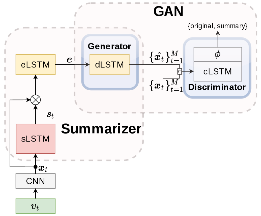
Conceptually, the model consists of four networks: selector LSTM (sLSTM), encoder LSTM (eLSTM), decoder LSTM (eLSTM), and discriminator LSTM (dLSTM). Note that we use LSTM models since we are dealing with sequential inputs. The figure below illustrates how SUM-GAN works. As an additional pre-processing step, given a video \(v_t\), SUM-GAN passes each of the frames into some pre-trained CNN \(\phi\) and encode them into a lower dimensional feature space \(x_t\). The sLSTM first takes \(x_t\) and maps then into normalized score \(s_t \in [0, 1]\). We then perform element-wise multiplication between \(x_t\) and \(s_t\) and encode the results into eLSTM to produce \(e\), where \(e\) is conceptually a representation of the summarized video in the feature space. We then takes \(e\) as the input to our dSLTM - which is the generator network in the GAN framework - and produces a reconstruced frame representation \(\hat{x_t}\). Note that, in practice SUM-GAN implemented the encoder-decoder with a VAE-LSTM. The discriminator cLSTM is a binary classifier that tries to classify whether the input frames belongs to the “original” or “reconstructed” class.
For training, these models are trained end-to-end in unsupervised manner (i.e., no manual labellings are required for the importance score). For the training objectives:
- sLSTM + eLSTM try to minimize reconstruction loss + prior loss (since eLSTM + dLSTM is a VAE-LSTM), and a sparsity loss that encourages the summarizer to come up with shorter summary.
- dLSTM tries to minimize reconstruction and GAN losses.
- cLSTM tries to maximize GAN loss.
Here, the reconstruction loss is defined as
\[\mathcal{L}_{reconst} = \mathbb{E}[-\log p(\phi(x) \vert e)]\], where they assume \(p(\phi(x) \vert e) \propto \textrm{exp}(- \vert\vert\phi(x) - \phi(\hat{x})\vert\vert^2)\) (i.e., \(p(\phi(x) \vert e)\) is Gaussian). The GAN loss is
\[\mathcal{L}_{GAN} = \log (\textrm{cLSTM}(x)) + \log (1 - \textrm{cLSTM}(\hat{x})) + \log (1 - \textrm{cLSTM}(\hat{x}_p))\], where \(\hat{x}_p\) is a set of reconstructed frames using random scores \(s_p\) being passed into eLSTM. The final term in \(\mathcal{L}_{GAN}\) is introduced to regularize the training of the discriminator to make sure it can differentiate \(\hat{x}_p\) as “reconstructed” class. The sparsity loss is
\[\mathcal{L}_{sparsity} = \Big\vert\Big\vert \frac{1}{M} \sum_{t=1}^M s_t - \sigma \Big\vert\Big\vert_2\], where \(M\) is the number of input frames, and \(\sigma \in [0, 1]\) represents the percentage of frames we expect to see in the summary (e.g., usually set to 0.15). Optionally, SUM-GAN also experimented with diversity and keyframe regularization. However, to keep this article short, I will skip these additional terms, and encourage you to see the paper if you are interested.
NOTE
- I think the notation in the figure can cause a bit of a confusion. Here, I think it is more appropriate to denote a video as \(v\) rather than \(v_t\) since a video is a sequence of \(M\) frames and the subscript \(t\) usually denotes the time index of each frame in the video. I think the figure tries to suggest that we encode each of the frames in the video using the pretrained CNN. Same goes for \(x_t\) and \(s_t\). From my understanding, \(e\) is also a set of features (i.e., \(e = [e_1, e_2, \dots]\)) rather than a single vector.
Cycle-SUM
Paper: Yuan et al. (2019)
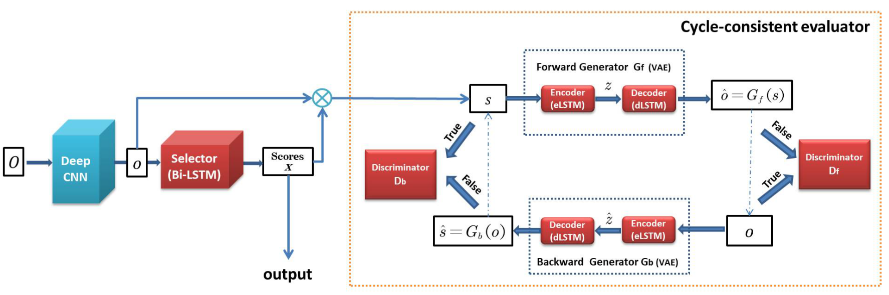
Cycle-SUM (Yuan et al., 2019) is another GAN-based method with the idea that a good video summary is the one that maximizes mutual information between the summarized and original video. This is concretised with a Cycle-GAN, which on top of the forward generator \(G_f\) and discriminator \(D_f\), is also equipped with a backward generator \(G_b\) and discriminator \(D_b\). As we see in the figure below, Cycle-SUM looks similar to SUM-GAN. The main difference is that now we have the backward generator and discriminator. Here, the backward generator maps a reconstructed video \(o\) to the summarized frame representation \(s\), and the backward discriminator classify whether the input is a true summary or not.
To train the models, Cycle-SUM optimizes the following loss function:
\[\mathcal{L} = \mathcal{L}_{sparsity} + \lambda_1(\mathcal{L}_{GAN,f} + \mathcal{L}_{GAN,b}) + \lambda_2(\mathcal{L}_{gen,f} + \mathcal{L}_{gen,b}) + \lambda_3 (\mathcal{L}_{cycle,f} + \mathcal{L}_{cycle,b})\]Here, \(\mathcal{L}_{sparsity}\) is the same sparsity loss that we see in SUM-GAN. Also, \(\mathcal{L}_{GAN,f}\) is the same GAN loss that we use in SUM-GAN, while \(\mathcal{L}_{GAN,b}\) is the backward version of it. Similarly, \(\mathcal{L}_{gen,f}\) is the same as the reconstruction loss we see in SUM-GAN, and \(\mathcal{L}_{gen,b}\) is just the backward version of it. We also notice additional objectives \(\mathcal{L}_{cycle,f}\) and \(\mathcal{L}_{cycle,b}\). With these loss terms, Cycle-SUM ensures that \(G_b(G_f(s)) = s\) and \(G_f(G_b(o)) = o\). Concretely, we define them as:
\[\mathcal{L}_{cycle,f} = \vert\vert G_b(G_f(s)) - s \vert\vert\] \[\mathcal{L}_{cycle,b} = \vert\vert G_f(G_b(o)) - o \vert\vert\]Finally, \((\lambda_1, \lambda_2, \lambda_3)\) are hyperparameters to weigh each of the loss terms.
During test time, we can take the output of the selector network, discretize them, and pick the ones with score equal to one as the selected keyframes.
CSNet
Paper: Jung et al. (2019)
Jung et al. (2019) propose a summarizer network with an attention mechanism called the CSNet. Overall, CSNet still follow the same framework in SUM-GAN, with a main difference in the network that outputs the importance score (i.e., sLSTM in SUM-GAN). The idea is to provide the model with global and local views of the input features so the model can deal with longer videos using chunk and stride mechanisms.
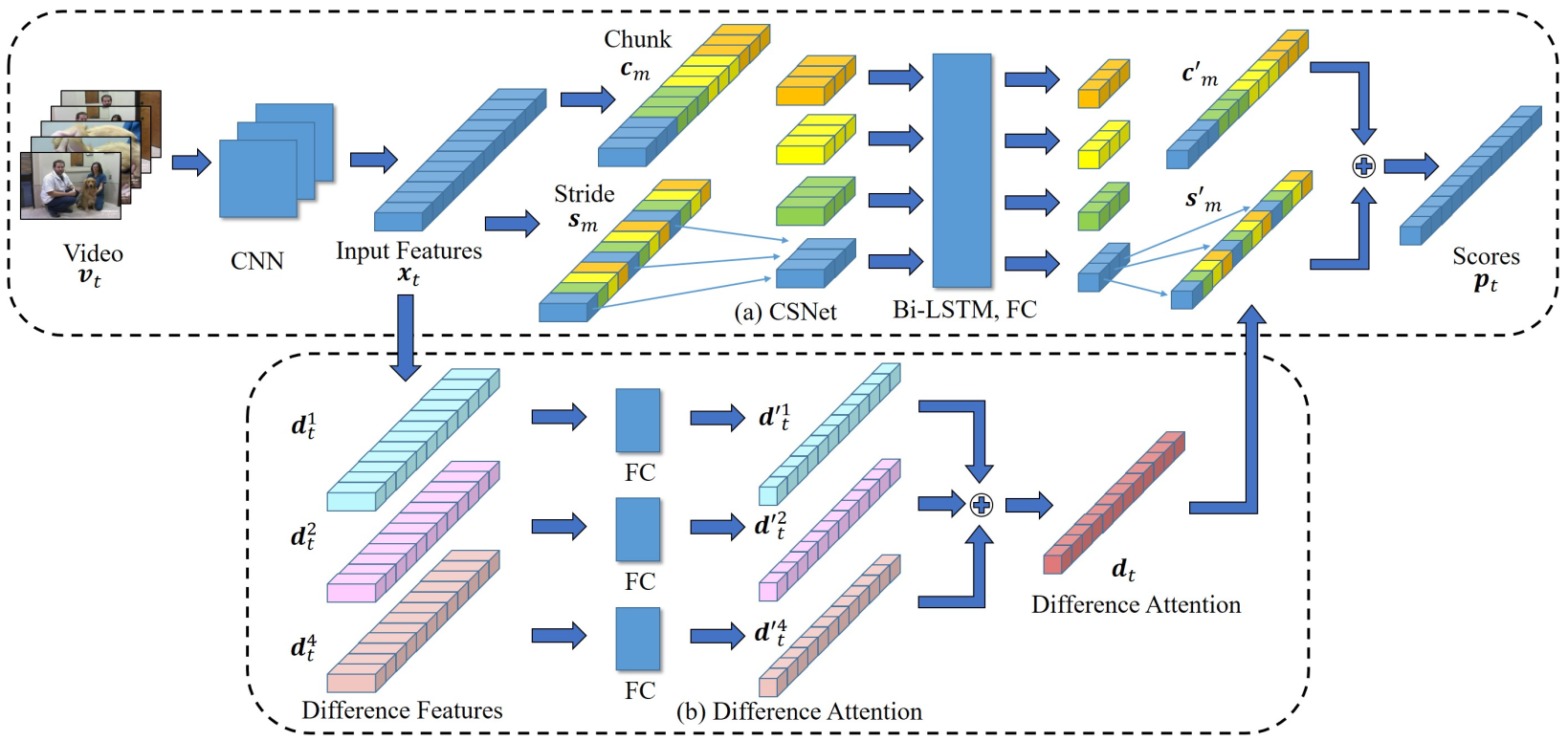
We can see illustration of CSNet in the figure below. Given an input features \(x_t\), the chunk mechanism divides \(x_t\) into multiple segments of successive features (color-coded in the figure). For example, if the input features are \([x_1, x_2, \dots, x_{12}]\), where each \(x_i\) denotes the frame representation at each time step, then the output of applying chunk mechanism may look something like \([x_1, x_2, x_3], [x_4, x_5, x_6], [x_7, x_8, x_9], [x_{10}, x_{11}, x_{12}]\). On the other hand, the stride mechanism segments \(x_t\) at uniform interval. For example, if the input features are \([x_1, x_2, \dots, x_{12}]\), after applying the stride mechanism, we may get something like \([x_1, x_5, x_9], [x_2, x_6, x_{10}], [x_3, x_7, x_{11}], [x_4, x_8, x_{12}]\). These segments are then passed to the summarizer network (i.e., in this case, this is the Bi-LSTM network) based on their temporal order. I would recommend to look at the figure since they are color-coded. The outputs of the Bi-LSTM are also reordered based on how we perform the chunk and stride to produce \(c'_m\) and \(s'_m\).
In addition, CSNet also employs difference attention mechanism by computing the difference between successive features, encoding them with some fully connected neural networks, and added them together to form a “difference attention” \(d_t\), which will then be used as a contributing factor to the scores \(p_t\). For example, in the paper, they compute the difference features \(d^i_t\) as:
\[d^1_t = \vert x_{t+1} - x_{t} \vert\] \[d^2_t = \vert x_{t+2} - x_{t} \vert\] \[d^4_t = \vert x_{t+4} - x_{t} \vert\]We can then compute \(d_t = d'^1_{t} + d'^2_{t} + d'^4_{t}\), where \(d'^1_{t} = FC(d^1_t)\), \(d'^2_{t} = FC(d^2_t)\), and \(d'^4_{t} = FC(d^4_t)\).
Finally, they also introduce a variance loss to prevent having flat distribution of importance score. Concretely, the variance loss is:
\[\mathcal{L}_{V}(p) = \frac{1}{\hat{V}(p) + \epsilon}\] \[\hat{V}(p) = \frac{\sum_{t=1}^T \vert p_t - median(p) \vert^2}{T}\]DSN with RL
Paper: Zhou et al. (2018)
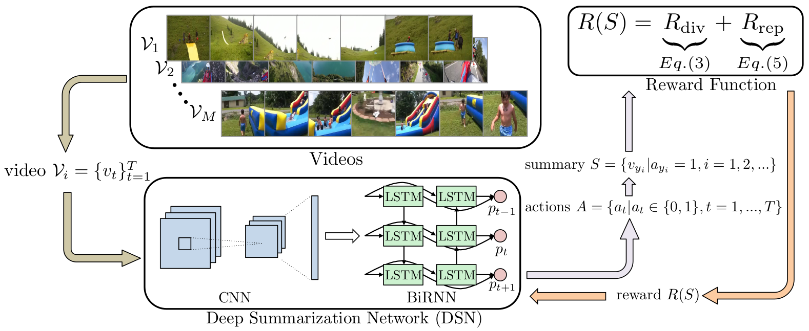
Unlike other approaches we discussed previously, Zhou et al. (2018) frame video summarization as a sequential decision problem and solve it using reinforcement learning (RL). The method is simply referred as deep summarization network (DSN), but we will refer this as DSN-RL instead, so we know that it is the method that uses RL. To summarize a video, DSN-RL trains a summarizer network with policy gradient method (i.e., REINFORCE), and designs a reward function based on heuristics. As we see in below figure, the policy network is a BiRNN that outputs importance score \(p \in [0, 1]\) of each input frames.
The first reward is based on the diversity of the selected keyframes:
\[R_{div} = \frac{1}{\vert \mathcal{Y} \vert (\vert \mathcal{Y} \vert - 1)} \sum_{t \in \mathcal{Y}} \sum_{t' \in \mathcal{Y}, t' \neq t} d(x_t, x_{t'})\] \[d(x_t, x_{t'})= \begin{cases} 1,& \text{if } \vert t' - t \vert > \lambda\\ 1 - \frac{x_t^T x_{t'}}{\vert\vert x_t \vert\vert_2 \vert\vert x_{t'} \vert\vert_2}, & \text{otherwise} \end{cases}\], where \(\mathcal{Y}\) denotes the set of selected keyframes time indeces, and \(\lambda\) is a threshold value for the temporal distance. By maximizing this reward, it encourages a solution where the keyframes are visually diverse. However, since we may encounter similar key events in different time, the reward is set to 1 if the temporal distance between two frames are higher than \(\lambda\). The second reward is based on the representativeness of the selected keyframes. The goal of this reward is to encourage a solution where the selected keyframes represent the original video. Concretely, this is defined as:
\[R_{rep} = \textrm{exp}(-\frac{1}{T} \sum_{t=1}^T \min_{t' \in \mathcal{Y}} \vert\vert x_t - x_{t'} \vert\vert_2)\]Summary
Currently, seems like a common theme is to train a network that outputs a video summary using the framework of GAN. In addition to GAN loss, common choices for the training loss include sparsity and diversity losses. To deal with possibly a long video sequence, the use of attention mechanism seems to generally be helpful. Finally, other than GAN-based approaches, one can also train a summarizer model using RL with heuristic-based reward function, as in DSN-RL.
References
Evlampios Apostolidis, Eleni Adamantidou, Alexandros I. Metsai, Vasileios Mezaris, Ioannis Patras. Video Summarization Using Deep Neural Networks: A Survey. arXiv, 2021.
Behrooz Mahasseni, Michael Lam, Sinisa Todorovic. Unsupervised Video Summarization with Adversarial LSTM Networks. CVPR, 2017.
Li Yuan, Francis EH Tay, Ping Li, Li Zhou, Jiashi Feng. Cycle-SUM: Cycle-consistent Adversarial LSTM Networks for Unsupervised Video Summarization. AAAI, 2019.
Yunjae Jung, Donghyeon Cho, Dahun Kim, Sanghyun Woo, In So Kweon. Discriminative Feature Learning for Unsupervised Video Summarization. AAAI, 2019.
Kaiyang Zhou, Yu Qiao, Tao Xiang. Deep Reinforcement Learning for Unsupervised Video Summarization with Diversity-Representativeness Reward. AAAI, 2018.