Long-Horizon Visual Planning with Goal-Conditioned Hierarchical Predictors
Paper: https://arxiv.org/abs/2006.13205
Disclaimer: I wrote this summary to the best of my understanding of the paper. I may make mistakes, so if you think my understanding of the paper is wrong, or if there is a typo or some other errors, please feel free to let me know and I will update this article.
Pertsch et al. (2020) propose a method called Goal-Conditioned Prediction (GCP) to perform visual planning by training a model that, given an image that an agent currently observes and a goal image, can produce possible trajectories to the goal location. There are multiple variations of the proposed method, but we will just focus on the hierarchical variation of it (i.e., GCP-Tree).
GCP-Tree
Given initial and goal images, the idea of GCP-Tree is to iteratively producing intermediate latent state between two parent states. Given \(o_1\) and \(o_T\), we first encode them into \(s_1\) and \(s_T\). We then need a model that produces the latent state that is supposedly halfway in time between the parent states. At the beginning, the parent states are \(s_1\) and \(s_T\), and we will use them to produce \(s_{\frac{T}{2}}\). In the next iteration, we apply the model again but to the new set of parent states. This time, the new set of parents are \((s_1, s_{\frac{T}{2}})\) and \((s_{\frac{T}{2}}, s_T)\), so we will produce \(s_{\frac{T}{4}}\), and \(s_{\frac{3T}{4}}\). We then keep repeating this until we have all the states \((s_1, ..., s_T)\). The figure below illustrates how GCP-Tree produces a sequence of images between \(o_1\) and \(o_T\).

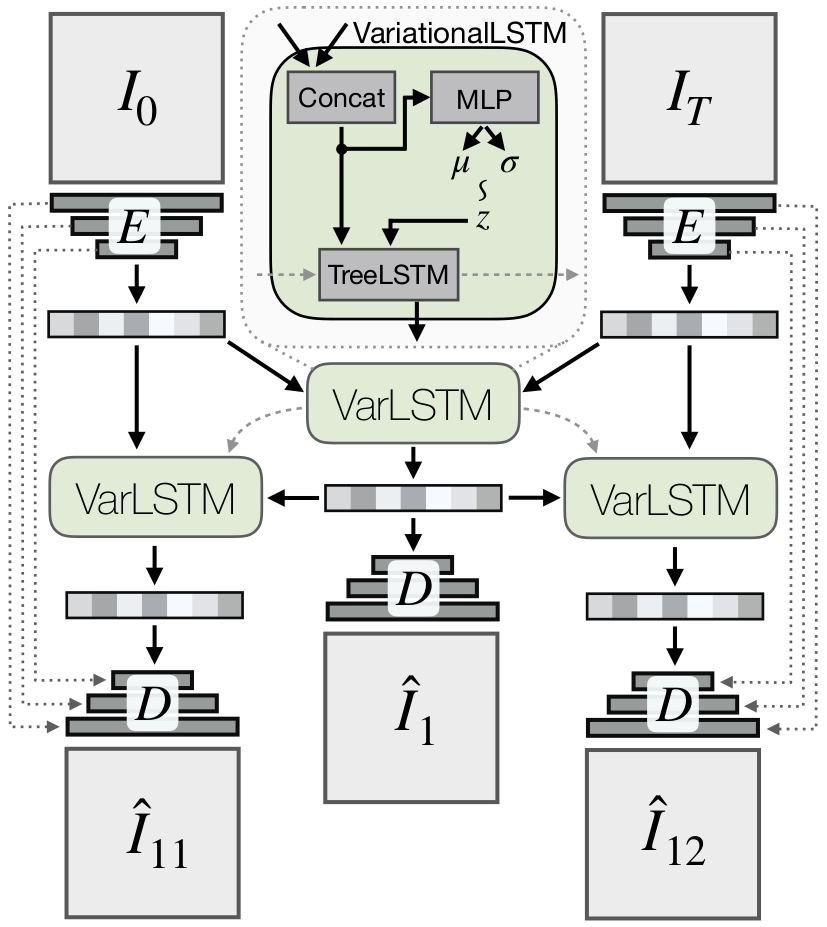
Concretely, GCP-Tree is realized with an encoder \(E\) that maps an image to some representation, a decoder \(D\) that maps some representation back into an image, and a variational LSTM (VarLSTM) that serves as a latent variable model for GCP. The figure below illustrates the model. First, given \(I_0\) and \(I_T\), we encode them using the encoder \(E\) to get some representation of it (let’s call them \(e_0\) and \(e_T\)). We then pass these two vectors into the VarLSTM module, where we will concatenate them into one vector. This concatenated vector is then passed into an MLP which will output parameters of the Gaussian \((\mu, \sigma)\), where we will sample the latent variable \(z\) from. We then pass the concatenated vector and \(z\) into the TreeLSTM to produce the output of VarLSTM module (let’s call it \(\hat{e}_{\frac{T}{2}}\)). In the next time step, we take \(e_{\frac{T}{2}}\), and obtain \(\hat{e}_{\frac{T}{4}}\) = VarLSTM(\(e_0\), \(e_{\frac{T}{2}}\)) and \(\hat{e}_{\frac{3T}{4}}\) = VarLSTM(\(e_{\frac{T}{2}}\), \(e_T\)), and keep repeating this until we have filled the space in between \(I_0\) and \(I_T\). To get the images, we just need to pass the output of the VarLSTM module at each time step to the decoder \(D\). In practice, they use some skip connections between the encoder and the decoder, as seen in the figure. To train this model, we can collect a dataset of an agent performing a task of interest in an environment, where the demonstration does not have to be optimal.
NOTE
Questions:
-
How do we know when to stop generating images? Do we need to know \(T\) in advance?
-
Seems like the model can only memorize a specific environment? For example, in the navigation example, seems like in order for it to work on a specific room layout, we need to train a model on a dataset obtained by the agent from the same room layout.
GCP with Adaptive Binding
I am actually interested to know more about how this works. The paper discusses how we can get images that correspond to keyframes (they call these as “semantic bottlenecks” in their paper) by doing this. For example, if the agent is planning to move an object to a particular bin, we may get an image of the agent is about to drop the object within the predicted plan. While there are some discussions on how this is done, I cannot figure out how exactly they are doing it. Perhaps I need to read this part more carefully.
Planning with GCP
Conceptually, we can perform planning with GCP by sampling multiple trajectories from a trained GCP model. To evaluate how good a trajectory is, we need to define some kind of cost function \(C(\cdot)\) that reflects how we want our agent to behave. We can then perform optimization to find the trajectory that minimizes the cost function. I will skip this part of the paper for now.
References
Karl Pertsch, Oleh Rybkin, Frederik Ebert, Chelsea Finn, Dinesh Jayaraman, Sergey Levine. Long-Horizon Visual Planning with Goal-Conditioned Hierarchical Predictors. NeurIPS, 2020.