Keyframing the Future: Keyframe Discovery for Visual Prediction and Planning
Paper: https://arxiv.org/abs/1904.05869
Disclaimer: I wrote this summary to the best of my understanding of the paper. I may make mistakes, so if you think my understanding of the paper is wrong, or if there is a typo or some other errors, please feel free to let me know and I will update this article.
Pertsch et al. (2020) propose a keyframe selection method called KeyIn by training two models. In this paper, keyframe selection is defined as finding \(N\) important frames \(K^{1:N}\) from a given sequence of frames \(I = I_{1:T} = [I_1, ..., I_T]\), as well as the corresponding time step of their appearances in the input sequence \(\tau^{1:N}\). To do this KeyIn trains an inpainting model and a keyframe predictor.

Inpainting model
Given two keyframes, the inpainting model is trained to generate sequence of images in between these keyframes. So, the inpainter is essentially performing interpolation in the image space. Concretely, given two adjacent keyframes \(K^n\) and \(K^{n+1}\) where \(1 \leq n \leq N\), and temporal distance between them (i.e., \(\tau^{n+1} - \tau^{n}\)), the model outputs sequence of images \(\hat{I}_{\tau^n:\tau^{n+1}-1}\). Since the output of the inpainter is a sequence of images, LSTM is naturally a good option for this model. We can train the inpainter in a purely supervised manner. Given an image sequence, we can sample two keyframes at random, and take all of the in-between images as the target images for the inpainter, and train the inpainter to minimize the \(L_1\) or \(L_2\) loss between the predicted and the target images.
Keyframe predictor model
Conceptually, the keyframe predictor is also an LSTM model that takes image sequence \(I = I_{1:T} = [I_1, ..., I_T]\) and generates keyframes \(K^{1:N}\) and the time index associated for each keyframes \(\tau^{1:N}\). However, for each keyframe \(K^n\), the model actually predicts the time offset from the previous keyframe \(\delta^n\). Furthermore, rather than predicting an integer, they represent \(\delta^n\) as a multinomial distribution (i.e., each element in \(\delta^n\) represents probability that \(K^n\) appears at a certain offset from \(K^{n-1}\)), and set a maximum offset of \(J\), so each \(\delta^n\) is a vector of length \(J\).
To train the keyframe predictor, we need to somehow compute the error for the predicted keyframes \(\hat{K}^{1:N}\) and the predicted offset \(\delta^{1:N}\). If we have a sequence of images labeled with the location of each keyframe, can we directly just minimize the reconstruction loss (e.g., \(L_2\) loss in image space) and the offset loss (i.e., cross-entropy loss)? Probably not a good idea, since the keyframe selection should be related to the offset prediction. Instead, KeyIn computes the expected target keyframe by computing the weighted sum of the input images \(\tilde{K}^n = \sum_{t}^{T} \tau^n_t I_t\), where \(\tau^n_t\) denotes the probability of \(K^n\) to be located at index \(t\). Since the model outputs the offset \(\delta^n\), we need to convert the predicted \(\delta^n\) into \(\tau^n\) (where \(\tau^n\) is a vector of length \(T\), and each element in it corresponds to \(\tau^n_t\)), where
\[\tau^n_t = \sum_{j} \tau^{n-1}_{t-j+1} \delta^n_j\]NOTE
In the paper, they wrote \(\tau^n_t = \sum_{j} \tau^{n-1}_{n-j+1} \delta^n_j\). However, I think this is a typo and it should be \(\tau^n_t = \sum_{j} \tau^{n-1}_{t-j+1} \delta^n_j\).
They also define \(c^n = \sum_{t}^{T} \tau^n_t\) to be the “probabilities of keyframes being within the predicted sequence”. The keyframe prediction loss is then defined as:
\[\mathcal{L}_{key} = \frac{\sum_{n}^{N} c^n \|\hat{K}^n - \tilde{K}^n\|^2}{\sum_{n}^{N} c^n}.\]NOTE
The keyframe prediction loss \(\mathcal{L}_{key}\) above is defined following Algorithm 1 in the paper. However, if we see Eq. 4 in the paper, \(\mathcal{L}_{key}\) is defined as
\[\mathcal{L_{key}} = \frac{\sum_{n}^{N} c^n \Bigg(\|\hat{K}^{n} - \tilde{K}^{n}\|^2 + \beta D_{KL} \Big(q(z^n \vert I, I_{CO}, z^{1:n-1}) \| p(z^n)\Big) \Bigg)}{\sum_{n}^{N} c^n}\]where \(q(\cdot)\) is the encoder part of the model that maps the input to a latent variable \(z\), and \(p(z)\) is the prior distribution (e.g., usually assumed to be Gaussian). So the KL divergence term is similar to the encoder loss when training a Variational Autoencoders (VAE). In the paper, they define \(I_{CO}\) as the “conditioning frames”. However, I am not sure how \(I = I_{1:T}\) and \(I_{CO}\) are different from each other.
Also, at this point, I am not actually sure if \(\tau^n_t\) and \(c^n\) are valid probability values. As I understand it, they still function to weigh the contribution of each keyframe prediction error to the loss function. They did say in the paper “Note that we efficiently implement computing of the cumulative distributions \(\tau\) as a convolution, which allows us to vectorize much of the computation.” So perhaps they are indeed some valid probability values.
In addition to \(\mathcal{L}_{key}\), we are also going to make sure that the inpainter is able to reconstruct the sequence from the predicted keyframes. Thus, when training the keyframe predictor, we freeze the inpainter model, and add the inpainting loss function to be part of the total loss.
In this case, the inpainting loss is computed as the following. First, they define \(e^n_j = \sum_{j > i} \delta^n_j\) to be “probabilities of segments ending after particular frames”, where \(i\) denotes the \(i\)-th index of the generated image from the \(n\)-th segment in \(\hat{I}^n_i\) (note that for each keyframe pairs, our inpainting model generates at most \(J\) frames). So, here, \(\hat{I}^n\) denotes the generated images at the \(n\)-th segment (which may contain up to \(J\) frames), and the subscript \(i\) denotes the index of the frame within this segment. They then define the “distributions of individual frames’ timesteps” as \(m^n_{j,t} \propto \tau^{n-1}_{t-j+1} e^n_j\) (or as they also mentioned, the “probability that the \(j\)-th predicted image in the \(n\)-th segment has an offset of \(t\) from the beginning of the predicted sequence.”), and compute the inpainting target as \(\tilde{I}_t = \frac{\sum_{n,j} m^n_{j,t} \hat{I}^n_j}{\sum_{n,j} m^n_{j,t}}\).
The inpainting loss is then defined as
\[\mathcal{L_{inpanting}} = \sum_{t}^{T} \|I_t - \tilde{I_t}\|^2\]So the total loss is \(\mathcal{L_{total}} = \mathcal{L_{key}} + \beta_{I} \mathcal{L_{inpanting}}\), where \(\beta_{I}\) denotes a hyperparameter to weigh the inpanting loss term.
The algorithm below (taken from the paper) shows how KeyIn computes the training loss.
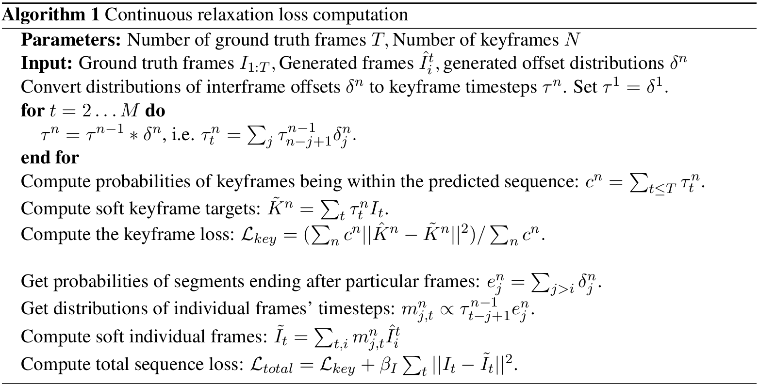
NOTE
In the above algorithm, the generated frames are denoted as \(\hat{I}^t_i\). I think it makes more sense to denote them as \(\hat{I}^n_i\) or \(\hat{I}^n_j\) (see above where we discuss about the inpainting loss for the keyframe prediction model). In addition, seems like there is inconsistency in the notation for computing the inpainting target where here they define \(\tilde{I}_t = \sum_{t,i} m^n_{j,t} \hat{I}^t_i\). I think it should be \(\tilde{I}_t = \frac{\sum_{n,j} m^n_{j,t} \hat{I}^n_j}{\sum_{n,j} m^n_{j,t}}\).
KeyIn for planning
I will skip this part of the paper for now. At the time of reading this paper, I was more interested in the keyframe prediction part.
References
Karl Pertsch, Oleh Rybkin, Jingyun Yang, Shenghao Zhou, Konstantinos G. Derpanis, Kostas Daniilidis, Joseph Lim, Andrew Jaegle. Keyframing the Future: Keyframe Discovery for Visual Prediction and Planning. L4DC, 2020.