Adaptive Skip Intervals: Temporal Abstraction for Recurrent Dynamical Models
Paper: https://arxiv.org/abs/1808.04768
Disclaimer: I wrote this summary to the best of my understanding of the paper. I may make mistakes, so if you think my understanding of the paper is wrong, or if there is a typo or some other errors, please feel free to let me know and I will update this article.
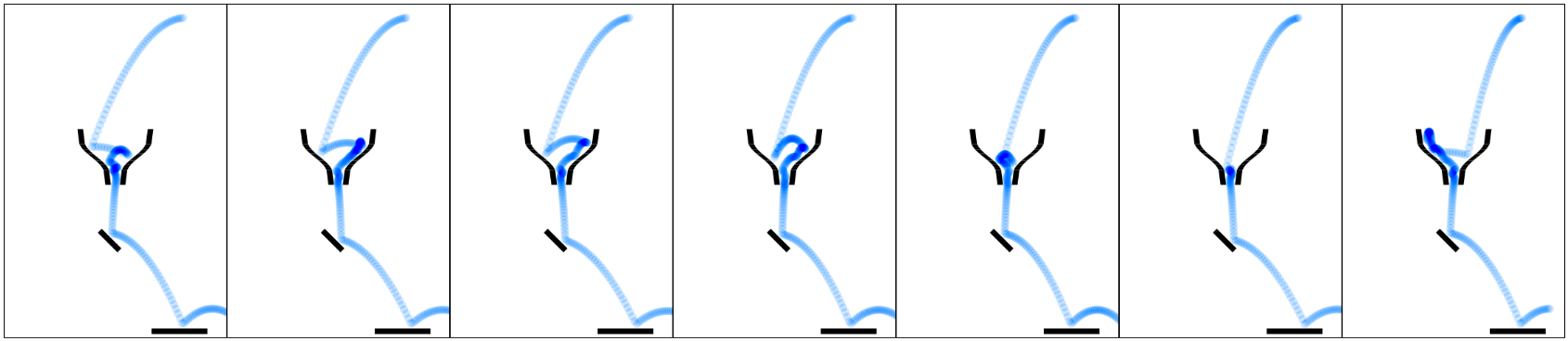
Neitz et al. (2018) propose a method to learn a dynamics prediction model by skipping states that do not matter. The idea is that we do not need to predict future states at every single step. Instead, it should really depends on what we are going to do with the predicted states. For example, the paper provides an example about ball being drop into a funnel as illustrated below. If all we care about is where the ball will land, then perhaps how the ball is bouncing inside the funnel does not matter. In all cases, the ball will eventually come out from the funnel and how the ball bounces inside the funnel should not affect where the ball will land. Thus, if we can somehow skip these transitions, the proposed method should be more efficient compared to methods that perform state prediction at every single step.
Concretely, Adaptive Skip Intervals (ASI) trains a neural network \(f\) that maps a state \(x_{t}\) to future state \(x_{t'}\) where the subscripts indicate the time step and \(t' > t\). ASI then define a horizon \(H\) to indicate the maximum number of future states that can be skipped (i.e., \(t' - t \leq H\)).
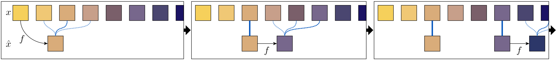
The figure below illustrates how ASI works. At the start, the model \(f\) takes the first state as an input and predicts a future state that is supposed to be within \(H\) time step away from the input state (here, they use \(H = 3\)). During training, ASI picks a ground truth state from the states that are \(H\) step away from the input state, and use it to compute the prediction loss (shown as solid blue line in the figure). At this point, let’s skip the details on how we pick this ground truth state, but we will discuss this later when we look at the algorithm. In this figure, for \(t \geq 2\) (assuming the sequence starts at \(t = 1\)), it looks like we always use the predicted state from previous time step as the input to the model. While this may be the case for test time, we will see soon how this is not exactly what we do when training the model.
The algorithm below shows how each training iteration is conducted. First, we take a dataset in the form of a sequence of states (i.e., a trajectory \(\mathbb{x} = (x_1, ..., x_T)\)). Starting from \(t = 1\), we take \(x_t\) and predict \(f(x_t) = \hat{x_u}\) so we can compute the prediction loss for the current time step (in the paper, the loss function that they use is the pixel-wise binary cross entropy). However, to compute the loss, we need to determine which state in the trajectory is the ground truth state for the prediction. There are two options to pick the ground truth state. The first one is via exploration, by randomly picking one of the states in \((x_{t+1}, ..., x_{t+H})\). The second is via exploitation by picking the state in \((x_{t+1}, ..., x_{t+H})\) that produces minimum loss (i.e., we need to compute the loss for \(\mathcal{L}(\hat{x_u}, x_{t+1}), ..., \mathcal{L}(\hat{x_u}, x_{t+H})\)). For each input, ASI picks the ground truth state via exploration with probability \(\mu\). Initially, the value of \(\mu\) is high to encourage exploration, but then it is decreased over time. After we compute the loss, we accumulate the loss in a variable \(l\) that will store the total loss for the entire trajectory. Note that we update the value of \(t\) when we pick the ground truth state. This is because we need to know where we currently are on the trajectory so we can determine which states are within the horizon \(H\). Before we move on to the next step, since we perform sequential prediction, for \(t \geq 2\), we can choose the input to the model to be either the ground truth state from the dataset \(x_t\) or the predicted state from the previous time step \(\hat{x_{u}}\). However, we cannot expect the model to perform well at the beginning of the training. Thus, ASI initially always uses the ground truth state as the input, and slowly moving to use the predicted state as the model improves over time. Concretely, ASI deploys schedule sampling strategy by picking to use the ground truth state with probability \(\epsilon\), where the value of \(\epsilon\) is decreased over time. These are then repeated until we have reached the end of the trajectory. We can then take the accumulated loss, compute the gradient of the accumulated loss with respect to the model parameters \(\theta\), and update \(\theta\).

References
Alexander Neitz, Giambattista Parascandolo, Stefan Bauer, and Bernhard Schölkopf. Adaptive Skip Intervals: Temporal Abstraction for Recurrent Dynamical Models. NeurIPS, 2018.